Keep it Simple, Stupid (KISS):

We’ve talked to businesses and economic development organizations about digitization, feelings about data, typical challenges with implementation of analytics, and the future adoption of machine learning / artificial intelligence. Previously, these struggles were discussed:

Incentives to digitalize early (or at all) in a small or micro business are quite small--especially if there is little realized return on investment due to an inability to derive insights from the data collected.
Data is expensive
Data is hard to collect and synthesize correctly
There isn't enough data
Data is not timely or difficult to keep timely

We set up Collective Vantage to combat these challenges in an easy, compelling, and affordable technology that spreads the load across networks of businesses that are onboarded. This post is going to detail a couple hour project that demonstrates just how effective a simple machine learning model can be for a micro/small business looking to understand how their future sales might look.

The Dataset:

For this project, we are using a retail dataset from Kaggle: https://www.kaggle.com/manjeetsingh/retaildataset . Since retail organizations are some of the most plentiful of the small/micro businesses at 2.6 million as of 2020 it makes sense to work on something related to retail.

What’s in this data?

We are given historical sales data for 45 stores located in different regions. The company runs several promotional markdown events throughout the year in their stores. These markdowns precede prominent holidays, the four largest of which are the Super Bowl, Labor Day, Thanksgiving, and Christmas. Store data and macro-economic dats is also provided as well.

What kind of Features are Included?

Contains additional data related to the store, department, and regional activity for the given dates.

Store Number
Date
Temperature
Fuel_Prices
MarkDown1-5 - % markdown amounts
CPI (Consumer Price Index)
Unemployment Rate
IsHoliday - True/False indicator of Holiday

What does the Sales Data Look Like?

Historical sales data, which covers to 2010-02-05 to 2012-11-01. Within this tab you will find the following fields:

Store Number
Department Number
Date
Sales Number

Yep, you can Collect this Data Yourself (and maybe already do)!

A theme when talking with small and micro business mentors is that most do not have reliable methods in place to collect operational and financial data. If you are reading this and head up a retail establishment, we hope to convey that tools like QuickBooks, Salesforce, Ecommerce Software, and many others can hold all of this very basic data. It is also quite easy to extract the data out of these systems for analysis. Even Excel can be a reliable when first starting out.

A key advantage to Collective Vantage is that the technology is designed around making data collection and aggregation easier across various tools used by businesses. It is often a daunting task to attempt this key step.

Onto Some Code!

Import the libraries we need

import pandas as pd
import numpy as np
import seaborn as sns
import sklearn
import matplotlib.pyplot as plt
import datetime
%matplotlib inline
from sklearn.ensemble import GradientBoostingRegressor,AdaBoostRegressor,RandomForestRegressor

Read in the data

store = pd.read_csv("store.csv")
feature = pd.read_csv("features.csv")
sales = pd.read_csv("sales.csv")

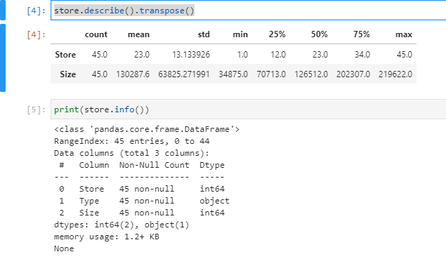
Get our bearings on what the structure of the data looks like for the store. We can see there is the store Id, Type, and the Size. Given that this is anonymized data, the values are somewhat non-sensical. However, the main concept is that these high-level data points can still be useful in prediction tasks. Plus, these can be very easy for a business to collect.

store.describe().transpose()

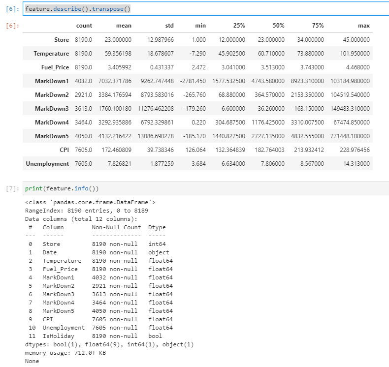
The features table holds good information about the store, markdowns, holidays, and macro-economic data. Again, all data that can easily be acquired, stored and used for analytics. The main thing to notice is that we have to clean up some of the blank fields.

feature.describe().transpose()

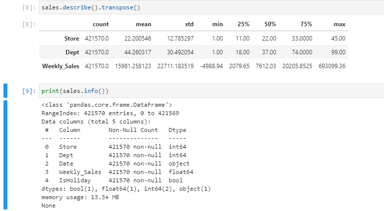
Finally, a cursory look at the sales data

Next step is to combine all the tables together to a single view

store_feat = store.merge(right = feature, on = 'Store')
df = store_feat.merge(right = sales, on = ['Store', 'Date', 'IsHoliday'])
df.sample(10)

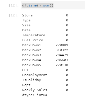
As mentioned previously, the first thing to tackle is making sure there are no blank records. In this project, if the week did not have a markdown, then the record is blank instead of 0. Since there is likely information in the weeks with and without markdown we will simply fill the blanks with 0’s.

df.isna().sum()
df['MarkDown1'] = df['MarkDown1'].fillna(0)
df['MarkDown2'] = df['MarkDown2'].fillna(0)
df['MarkDown3'] = df['MarkDown3'].fillna(0)
df['MarkDown4'] = df['MarkDown4'].fillna(0)
df['MarkDown5'] = df['MarkDown5'].fillna(0)

Next some features will be created to derive more information from the dimensions that already exist:

def day_of_year(date_str):
    date = datetime.datetime.strptime(date_str, '%d/%m/%Y')
    return date.timetuple().tm_yday

def day(date_str):
    date = datetime.datetime.strptime(date_str, '%d/%m/%Y')
    return date.timetuple().tm_mon

def year(date_str):
    date = datetime.datetime.strptime(date_str, '%d/%m/%Y')
    return date.timetuple().tm_year

def woy(date_str):
    date = datetime.datetime.strptime(date_str, '%d/%m/%Y')
    return date.timetuple().tm_year

df['DayOfYear'] = df['Date'].map(day_of_year)
df['MonthOfYear'] = df['Date'].map(day)
df['Year'] = df['Date'].map(year)
df['DayOfYearCos'] = np.cos(df['DayOfYear'])
df['DayOfYearSin'] = np.sin(df['DayOfYear'])
df['Date'] = pd.to_datetime(df['Date'])
df["WeekofYear"] = df.Date.dt.week

df['IsHoliday'] = df['IsHoliday'].astype('category')
df['Dept'] = df['Dept'].astype('category')
df['Store'] = df['Store'].astype('category')

Some key things to note on the features created with the code above:

Deconstruct the date to get the year, day, month, and week of the year to make sure we increase the opportunity for our model to pick up on trends—hopefully increasing predictive power
Calculate the Sin and Cosine of the day of the year as these features help maximize our ability to fit the cyclical nature of the retail data
- https://medium.com/swlh/time-series-forecasting-with-a-twist-27350e97a2cb
- https://towardsdatascience.com/cyclical-features-encoding-its-about-time-ce23581845ca
- https://towardsdatascience.com/taking-seasonality-into-consideration-for-time-series-analysis-4e1f4fbb768f
Convert the IsHoliday, Dept, and Store dimensions to categories so they may be encoded using pd.get_dummies. Department and Store are given an ordinal encoding in the dataset. Because these encodings represent unique categories we do not want the ordinal nature of the encodings to be picked up by the algorithm since these data really should be totally distinct. The Department dimension should be treated along the same lines

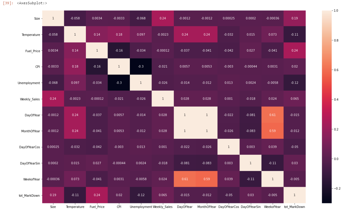
After the cleaning the data and creating some additional features, visualizing the data highlights some key things to keep in mind later. Firstly, a correlation plot is generated to assess how each of the variables are correlated with each other—not to be confused with causation.

df_temp = df.copy(deep=True)
df_temp['tot_MarkDown'] = df_temp['MarkDown1'] + df_temp['MarkDown2'] +df_temp['MarkDown3'] +df_temp['MarkDown4'] + df_temp['MarkDown5']
df_temp.drop(['MarkDown1', 'MarkDown2', 'MarkDown3', 'MarkDown4', 'MarkDown5','Year'], inplace = True, axis = 1)
fig, ax = plt.subplots(figsize=(20,12))
sns.heatmap(df_temp.corr(),annot=True)
# df_temp.head

There are not a ton of highly correlated features in this dataset. MonthOfYear and DayOfYear are going to be somewhat correlated.

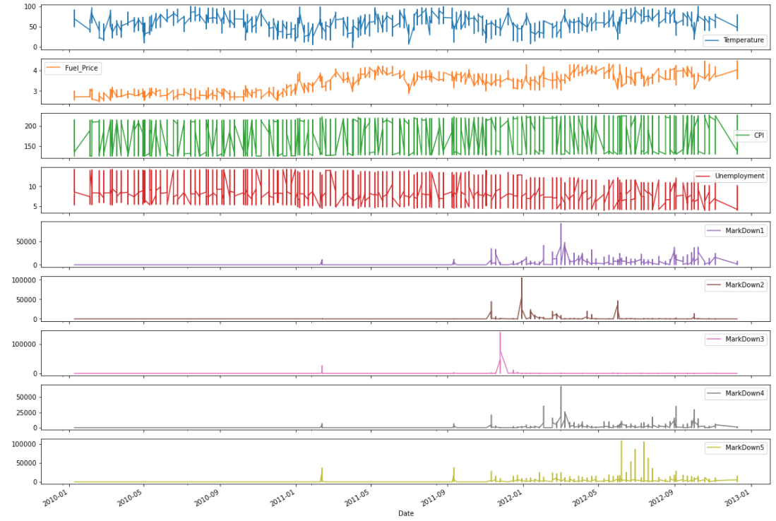
The next chart looks at the timeseries data to establish an understanding of how the trends relate:

df[['Date', 'Temperature', 'Fuel_Price', 'CPI', 'Unemployment', 
    'MarkDown1', 'MarkDown2', 'MarkDown3', 'MarkDown4', 'MarkDown5']].plot(x='Date', subplots=True, figsize=(20,15))
plt.show()

It is easy to notice that there really aren’t a ton of variables that trend along the sales cycle. A lack of observable trend is not necessarily a problem, but it certainly makes the model more abstract and potentially less interpretable. What is great about machine learning, the obscure connections between various inputs can be found and exploited to produce awesome insights—a level of inference that human intuition just can’t have without extensive time and effort.

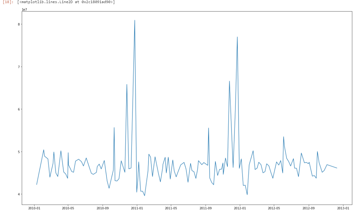
Next, visualize the weekly sales numbers over time to get a closer look at the sales over time:

df_time = df.groupby('Date').sum()['Weekly_Sales'].reset_index()
fig, ax = plt.subplots(figsize=(20,12))
ax.plot('Date', 'Weekly_Sales', data=df_time)

A closer look reveals more of the cyclical nature of the sales over time. Dips in sales seems to occur just after the New Year, but peak around Christmas, Thanksgiving, Memorial Day, and 4th of July. So, pretty typical sales behavior from a retail establishment. Funnily enough, the trend also looks like a WAVE! T

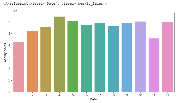
Furthermore, the seasonality can be further visualized by looking at the sales split by month:

df_seas = df.groupby(df.Date.apply(lambda x: x.month)).sum()['Weekly_Sales'].reset_index()
plt.figure(figsize=(10, 5))
sns.barplot(x=df_seas.Date,y=df_seas.Weekly_Sales)

Interesting the peaks in April and December.. The dips in January and November are also interesting given that the largest peaks in the sales timeseries charts.

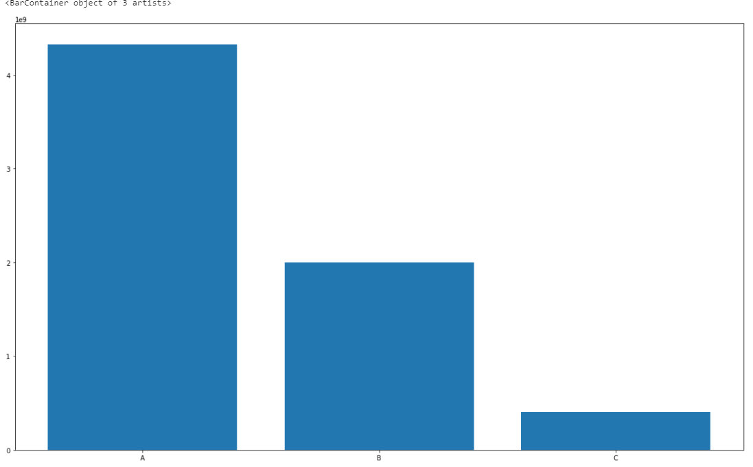
Finally, the sales by store type will be visualized:

df_store_type = df.groupby('Type').sum()['Weekly_Sales'].reset_index()
fig, ax = plt.subplots(figsize=(20,12))
ax.bar('Type', 'Weekly_Sales', data=df_store_type)

Interesting to note here that Store Type A has a significant advantage over Types B and C in terms of predictive capability because of the amount of sales is not distributed evenly. The model we will develop will include sales from all the store types. In the future, it might be useful to develop a model specific to each store type.

Data preparation for modeling is next:

model = df.set_index(['Date', 'Store', 'Dept']).sort_index()
model_data = model.reset_index()
from sklearn.preprocessing import MinMaxScaler

mms = MinMaxScaler()
model_data[['Temperature','Fuel_Price','MarkDown1','MarkDown2',
            'MarkDown3','MarkDown4','MarkDown5','CPI','Unemployment',
            'Size']] = mms.fit_transform(model_data[['Temperature','Fuel_Price','MarkDown1','MarkDown2',
                                                     'MarkDown3','MarkDown4','MarkDown5','CPI',
                                                     'Unemployment','Size']])

model_data = pd.get_dummies(model_data,drop_first=True)
final_model = model_data.set_index('Date')

The block of code does a few key things:

Sort the table by the Date, Store and Department
Scale the numeric features down to between 0 and 1. This step is necessary in order to bring everything to the same scale

Splitting the data to a training and prediction set occurs next—in addition to defining the features and what we are actually trying to predict. Training will be used to evaluate the basic model and prediction will be used to test how good our model actually is on unseen observations:

training_model = final_model[:'2012-01-01']
training_model.reset_index(inplace=True)
pred = final_model['2012-01-01':]
pred.reset_index(inplace=True)
X_model_train = training_model.drop(columns=['Weekly_Sales', 'Year', 'DayOfYear','Date'])
y_model_train = training_model['Weekly_Sales']
X_pred = pred.drop(columns=['Weekly_Sales', 'Year', 'DayOfYear','Date'])
y_pred = pred['Weekly_Sales']

For this project, we are going to split the data a bit differently. Both training and prediction will be split into their own train and test sets.

from sklearn.model_selection import train_test_split

X_train, X_test, y_train, y_test = train_test_split(X_model_train, y_model_train, test_size=0.10, random_state=0)

Splitting the data allows us to then build the basic model that will be the benchmark. Gradient Boosting Regressors are one of my go-to algorithms from Sklearn because of the resilience to overfitting, tunability, and flexibility.

from sklearn.ensemble import GradientBoostingRegressor

gbr_regressor = GradientBoostingRegressor()

gbr_regressor = gbr_regressor.fit(X_train, y_train)
gbr_regressor.score(X_test, y_test)

future_pred = gbr_regressor.predict(X_pred)
gbr_regressor.score(X_pred, y_pred)

Training score = 0.697 (69%)
Test score = 0.743 (74%)
The base model mean squared error (MSE) on test set: $166,493,765.3
The base model mean absolute error (MAE) on test set: $8201.4
The base model root mean squared error (RMSE) on test set: $12,903.2

When looking at the scores for the Gradient Boosted Regressor, it is important to note that the Score is actually an R^2 value. The R^2 value is, generally, a metric that provides insight into how well the model fits the data. There’s lots of room for interpretability. Domain experience will dictate whether or not the model performs the fit well enough. In this project, the score is not terrible but might be able to be optimized. An area of concern is the assessment of the mean squared error, mean absolute error, and root mean squared error. A very high mean squared error indicates that there are significant errors that exist and can be problematic in future predictions. A Mean Absolute Error of $8201.4 seems to be acceptable, but would need to be evaluated by the stakeholders in the retail shop. RMSE is a less interpretable metric for accuracy. However, RMSE does a nice job of balancing the extreme errors against the more ‘normal’ prediction errors. There is definitely some room to improve.

Sklearn offers GridSearchCV and RandomizedSearchCV in order to test lots of parameters. GridSearchCV is very slow. RandomizedSearchCV is much faster and returns results faster:

from sklearn.model_selection import KFold
from sklearn.model_selection import RandomizedSearchCV

parameters = {'learning_rate':[0.05, 0.1, 0.5, 1], 
              'min_samples_split':[2,5,10], 
              'max_depth':[2,3,5],
             'n_estimators':[100,150,250]}

gbr_regressor = GradientBoostingRegressor()
cv_test= KFold(n_splits=5)
clf = RandomizedSearchCV(gbr_regressor, parameters,cv=cv_test,n_jobs=-1)
clf.fit(X_train, y_train)

{'n_estimators': 250, 'min_samples_split': 10, 'max_depth': 5, 'learning_rate': 0.5}

After about 30 min, the model returns the best parameters. The model can be re-run with the new parameters to get an accuracy score:

gbr_regressor_tuned = GradientBoostingRegressor(n_estimators = 250, 
                                                min_samples_split = 10, 
                                                max_depth = 5, 
                                                learning_rate = 0.5)

X_train_pred, X_test_pred, y_train_pred, y_test_pred = train_test_split(X_pred, y_pred, test_size=0.10, random_state=0)

gbr_regressor_tuned = gbr_regressor_tuned.fit(X_train_pred, y_train_pred)
gbr_regressor_tuned.score(X_test_pred, y_test_pred)

future_pred = gbr_regressor_tuned.predict(X_test_pred)
gbr_regressor_tuned.score(X_test_pred, y_test_pred)

Tuned Prediction Set Score 96.7%
The tuned model mean squared error (MSE) on prediction set: $16,116,078.3
The tuned model mean absolute error (MAE) on prediction set: $2,379.7
The tuned model root mean squared error (RMSE) on prediction set: $4,011.6

Note here that our R^2 jumped by over 20%. Depending on the use-case that type of increase can indicate over-fitting of the model. However, MSE, MAE, and RMSE all declined precipitously. The hyper-parameter tuning seems to have helped significantly with the predictive power of the model.

Cool, but why does this matter?

The ability, at least generally, to predict sales from week to week is hugely important in a tighter margin retail space—where the stakes are high:

Improve the ability to staff more efficiently
Purchase material in a more efficient way
Reduce the level of risk when planning financial and capital investments

Sorry, I just don’t have enough data to do this kind of Modeling!

For many businesses, there just won’t be enough data to build a model. Unfortunately, a vast majority of small/micro businesses simply will not have enough data. So what are these businesses supposed to do? What if you have a new business trying to forecast potential sales within a business community? Collective Vantage wants to eliminate the need to worry about these hurdles. Even if you only have a small amount of data, there are probably similar businesses to yours that probably already has enough to build a forecast.

Even if I had data to Forecast, I don’t know how to code or Productionize anything

Collective Vantage condenses the technical know-how to a manageable level. Conaxon brings the tech and the users bring the domain experience. It’s as simple as asking a question like: “What might my sales look like next week, month, year?”

Keep Analytics, Machine Learning, and Artificial Intelligence to Simple Use-Cases with Collective Vantage