Predict which Sales Leads Close Part 1
Setting the Stage:
Consider for a moment that your business is doing quite well. Sales is quickly climbing, the sales funnel is quite full, and customer service is top notch. But, because you are a responsible leader and manager the future appears somewhat hazy! Growth is wonderful, to be sure. However, growth can only scale as well as the sales team—and by extension, the rest of your operations. At some point the sales funnel will become exceedingly top heavy, business leaders will have to decide: do we hire more team members to support the increased demand or do we attempt to lean out somewhat so as to preserve margin, customer service, and specialization?
A tough, but highly personal choice.
I am willing to bet, a great many businesses would choose the option to lean out, maintain margins, and continue to develop productive their salespeople. There are a few pillars critical to projects where efficiency is the desired output, but maybe none more critical than tools. Having a diverse toolbox is essential. Data analytics and machine learning is quickly becoming an essential tool in the toolbox.
Proposed Solution:
All that said, I propose that machine learning could be used to predict which sales leads might close; therefore, allowing salespeople some insights into which leads should be prioritized first in the funnel. Secondarily, this algorithm could be used as a tool for identifying sales opportunities NOT being closed that may be critical now or in the future.
Business Context:
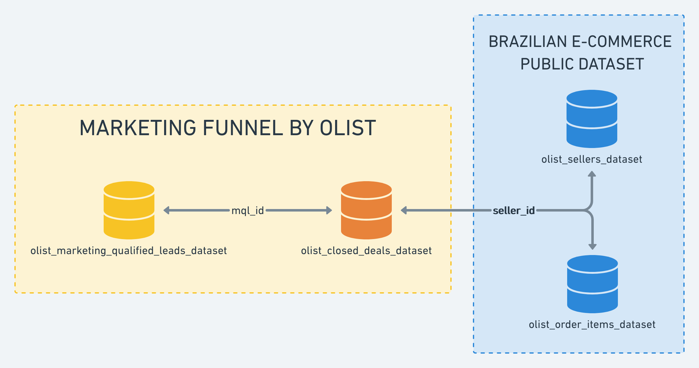
In order to demonstrate the capability of machine learning to address the aforementioned use case, we searched for a public dataset to perform tests. The team landed on a Kaggle dataset posted by a company called Olist—the largest department store in Brazilian marketplaces (link: https://www.kaggle.com/olistbr/marketing-funnel-olist?select=olist_marketing_qualified_leads_dataset.csv). This is a marketing funnel dataset from sellers that populated a form that requested to sell their products on the Olist Store. Olist connects small businesses from all over Brazil to channels without hassle and a single contract. Merchants are able to sell their products through the Olist Store and ship them directly to the customers using Olist’s supply chain partners.
The sales process is as follows:
Sign-up at a landing page
Sales development Representative (SDR) contacts lead, collects some information and schedules an additional consultancy
Consultancy is made by a Sales Representative (SR). The SR may close the deal or not
Lead becomes a seller and starts building their catalog on Olist
The products are published on Olist marketplaces and ready to sell!
The Dataset:
The dataset has information related to 8,000 Marketing Qualified Leads (MQLs) that requested a contact. these MQLs were randomly sampled from a larger set of MQLs.
The algorithm will use the data from the qualified leads daraset and closed leads dataset. A future projet might be demand/sales forecasting using the sellers dataset and order items dataset.
Jumping into the Data:
When testing, I like to use Jupyter Lab. I find it to be supremely easy to work with and lends itself to iteration, agility, and ease of use. First, we will import the libraries we will be using:
import pandas as pd
import seaborn as sns
import matplotlib.pyplot as plt
import numpy as np
from datetime import datetime
Now, we are going to read in the data for the analysis:
closed_deals = pd.read_csv('olist_closed_deals_dataset.csv')
olist_leads = pd.read_csv('olist_marketing_qualified_leads_dataset.csv')
Next, we are going to combine the qualified leads and the closed deals to create a single dataset for generating predictions. The documentation from Kaggle was really great so there is no mystery as to how the join needs to be performed.
funnel = pd.merge(olist_leads,closed_deals,how='left',on='mql_id')
The next lines of code are going to be adding some potentially useful features and removing others that won’t be useful in the prediction model. The code is pretty simple and self-explanatory. Initially, time-to-close was thought to be useful in the prediction, but at the time of writing the report the features were not used in the model. Time-to-close would likely be more important as a business analysis task rather than a prediction task. The code is left in this report for reference anyways:
funnel['won_date'] = funnel['won_date'].astype('datetime64[ns]')
funnel['first_contact_date'] = funnel['first_contact_date'].astype('datetime64[ns]')
funnel['time_to_close'] = funnel['won_date'] - funnel['first_contact_date']
funnel['time_to_close'] = funnel['time_to_close'].dt.days

funnel.drop('declared_monthly_revenue',axis=1,inplace=True)
funnel.drop('declared_product_catalog_size',axis=1,inplace=True)
funnel.drop('average_stock',axis=1,inplace=True)
funnel.drop('has_company',axis=1,inplace=True)
funnel.drop('seller_id',axis=1,inplace=True)
indexNames = funnel[ (funnel['time_to_close'] < 0)].index
funnel.drop(indexNames , inplace=True)
It is important to note that many of these dimensions were dropped because there was very little data to begin. There are instances of imputation later in the project that could have been applied to these dropped dimensions; however, there was little data to even be able to reliably impute from as a baseline.
The next line of code defines what we are going to end up trying to predict—a binary TRUE or FALSE classification:
funnel['closed_deal'] = funnel['won_date'].notnull()
This particular project did not attempt to understand time to close, but could easily be revisited at a later time.
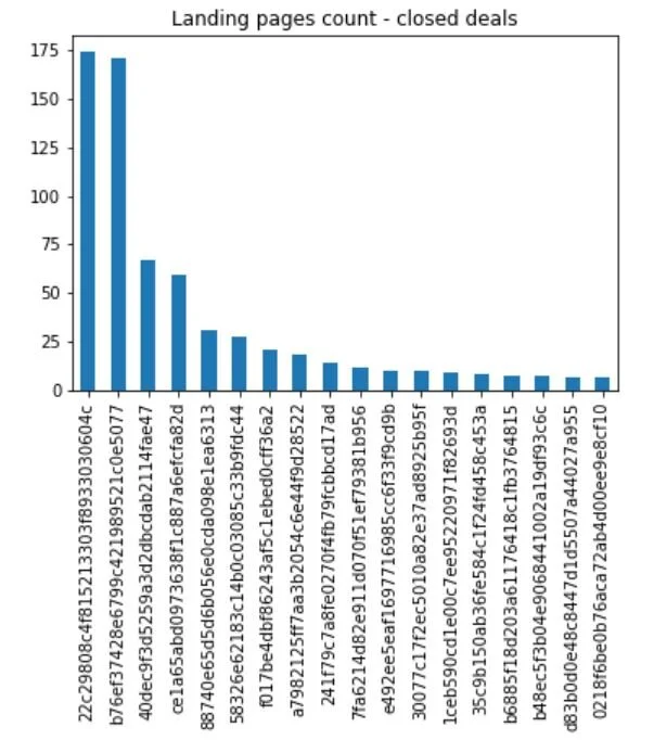
Each project typically starts with some basic exploratory data analysis. I want to have a devent understanding of the spread in time-to-close, which SRs and SDRs are closing most often, and which features might have the most importance in a prediction. Let’s start with a basic understanding of which landing pages seem to close the most deals:
pg_id = funnel.loc[funnel['closed_deal'] == True]
pg_id = pg_id.landing_page_id.value_counts()
pg_id[pg_id.values > 5].plot(kind="bar")
plt.title("Landing pages count - closed deals")
plt.savefig("landing_page_counts.png")
plt.show()
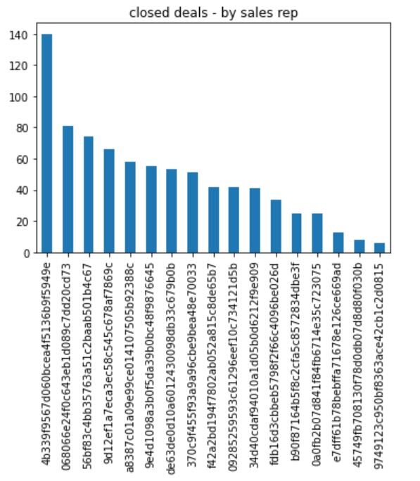
Next, it might be interesting whom are the most effective SRs:
sr = funnel.loc[funnel['closed_deal'] == True]
sr = sr.sr_id.value_counts()
sr[sr.values > 5].plot(kind="bar")
plt.title("closed deals - by sales rep")
plt.savefig("landing_page_counts.png")
plt.show()
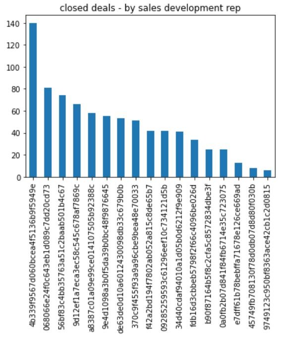
Next, we look at the most effective SDRs:
sdr = funnel.loc[funnel['closed_deal'] == True]
sdr = sdr.sdr_id.value_counts()
sdr[sdr.values > 5].plot(kind="bar")
plt.title("closed deals - by sales development rep")
plt.savefig("landing_page_counts.png")
plt.show()
We’ll finish off the exploratory data analysis with a cursory understanding of how long it takes to close a deal based on various features in the dataset. Again, this part of the business analysis is not strictly pertinent but potentially useful knowledge for further development. The business might find it useful in the future to have a prediction of when a deal might close—thereby allowing some ability to better understand potential revenue.
sns.displot(data=funnel, x="time_to_close", col="origin", kde=True,col_wrap=2)
sns.displot(data=funnel, x="time_to_close", col="business_segment", kde=True,col_wrap=2)
sns.displot(data=funnel, x="time_to_close", col="lead_type", kde=True,col_wrap=2)
sns.displot(data=funnel, x="time_to_close", col="business_type", kde=True,col_wrap=2)
Overall, the data analysis wasn’t too conclusive but gave decent exposure to some of the intricacies of the dataset. You’ll notice that in many areas, the data is quite sparse and not many samples to develop a robust model. It would be advisable, like in most instances, to acquire more data to test and fine tune hyper parameters.
After the brief data analysis, we can begin to further clean and develop the features going to be used in the prediction:
funnel_model = funnel.copy(deep=True)
funnel_model['contact_day'] = funnel_model['first_contact_date'].dt.strftime('%d')
funnel_model['contact_month'] = funnel_model['first_contact_date'].dt.strftime('%m')
funnel_model['contact_year'] = funnel_model['first_contact_date'].dt.year
funnel_model.drop('time_to_close',axis=1,inplace=True)
funnel_model.drop('won_date',axis=1,inplace=True)
funnel_model.drop('first_contact_date',axis=1,inplace=True)
funnel_model.drop('mql_id',axis=1,inplace=True)
funnel_model.drop_duplicates()
There are a few things to note with the preceding code:
Extract the contact day, month, and year because the date alone is not going to be a useful predictor
Drop the time to close (for the time being) as it will not be used in the initial model
Drop the date in which the contract was won. The date itself and it’s date components also will not be useful
Drop the first contact date as it will not be a useful predictor itself
Drop the unique qualified id because it is not useful
Drop any duplicates in the dataset so we ensure that bias is less likely
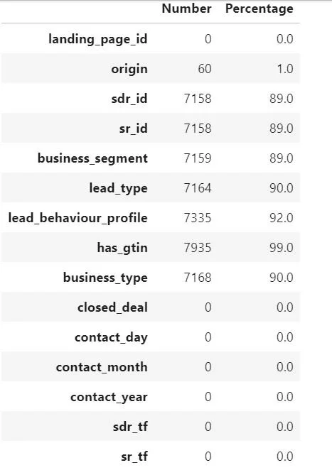
The following code addresses a particularly thorny problem from an architectural standpoint. There were a significant number of ‘na’ or ‘nan’ values with the combination of the close deals and leads dataset. In order to properly demonstrate the use case, the ‘na’ and ‘nan’ values will need to be addressed through imputation. In this investigation, we are going to assume that if the won date is null, then the contract has been lost—thereby giving us a population of leads not won and those that have been won (remember the line of code above: funnel['closed_deal'] = funnel['won_date'].notnull()). There is no other identifier for a lead in progress or otherwise.
A simple line of code to determine the number of ‘na’ and ‘nan’ records is the following:
#count missing values (NAs)
missing_count = pd.DataFrame(funnel_model.isna().sum(),columns=['Number'])
missing_count['Percentage'] = round(missing_count / len(funnel_model),2) * 100
missing_count
Given that there were so many missing feature values, imputation should be sufficient to demonstrate how to properly fill the gaps in the data model. Conceptually, the imputation employed was simple. A function was created to write the unique values from a feature to a list. Then, another line of code was written to randomly choose values from that list to fill the ‘na’ or ‘nan’ within the dimension:
origin_list = funnel_model["origin"].unique()
origin_list = [x for x in origin_list if str(x) != 'nan']
funnel_model['origin'] = funnel_model['origin'].fillna(pd.Series(np.random.choice(origin_list, size=len(funnel_model.index))))

sdr_id_list = funnel_model["sdr_id"].unique()
sdr_id_list = [x for x in sdr_id_list if str(x) != 'nan']
funnel_model['sdr_id'] = funnel_model['sdr_id'].fillna(pd.Series(np.random.choice(sdr_id_list, size=len(funnel_model.index))))

sr_id_list = funnel_model["sr_id"].unique()
sr_id_list = [x for x in sr_id_list if str(x) != 'nan']
funnel_model['sr_id'] = funnel_model['sr_id'].fillna(pd.Series(np.random.choice(sr_id_list, size=len(funnel_model.index))))

bs_list = funnel_model["business_segment"].unique()
bs_list = [x for x in bs_list if str(x) != 'nan']
funnel_model['business_segment'] = funnel_model['business_segment'].fillna(pd.Series(np.random.choice(bs_list, size=len(funnel_model.index))))

lead_list = funnel_model["lead_type"].unique()
lead_list = [x for x in lead_list if str(x) != 'nan']
funnel_model['lead_type'] = funnel_model['lead_type'].fillna(pd.Series(np.random.choice(lead_list, size=len(funnel_model.index))))

lbp_list = funnel_model["lead_behaviour_profile"].unique()
lbp_list = [x for x in lbp_list if str(x) != 'nan']
funnel_model['lead_behaviour_profile'] = funnel_model['lead_behaviour_profile'].fillna(pd.Series(np.random.choice(lbp_list, size=len(funnel_model.index))))

gtin_list = funnel_model["has_gtin"].unique()
gtin_list = [x for x in gtin_list if str(x) != 'nan']
funnel_model['has_gtin'] = funnel_model['has_gtin'].fillna(pd.Series(np.random.choice(gtin_list, size=len(funnel_model.index))))

btype_list = funnel_model["business_type"].unique()
btype_list = [x for x in btype_list if str(x) != 'nan']
funnel_model['business_type'] = funnel_model['business_type'].fillna(pd.Series(np.random.choice(btype_list, size=len(funnel_model.index))))
After filling the ‘nan’ and ‘na’ values, a combination between the SDR id and SR id to build a feature that uses the combo to predict closure:
funnel_model['sdr_sr'] = funnel_model['sdr_id'] + funnel_model['sr_id']
If we re-run the code for determining the ‘na’ or ‘nan’ value there should not be any left. You’ ll notice there is a single record still left ‘nan’ —so I drop it.
#count missing values (NAs)
missing_count = pd.DataFrame(funnel_model.isna().sum(),columns=['Number'])
missing_count['Percentage'] = round(missing_count / len(funnel_model),2) * 100
missing_count
funnel_model.loc[funnel_model['has_gtin'].isnull()]

funnel_model = funnel_model.drop(index=7999)
At this point, the data model should be set properly. First, we select the features to be used in the model. The next step will be to encode the categorical data. For this implementation, one-hot encoding was used as ordinal encoding did not seem to be appropriate.
df1 = funnel_model[['landing_page_id', 'origin', 'sdr_id','sr_id','business_segment',
                   'lead_type','lead_behaviour_profile','has_gtin','business_type','closed_deal',
                  'contact_day','contact_month','contact_year','sdr_sr']].copy()

pd.get_dummies(df1)

pd.get_dummies(df1.drop('closed_deal',axis=1),drop_first=True)
It was a long road to get here, but the following code will apply to model development. Support Vector Classifier and Decision Trees from Sci-kit Learn will be used initially for the prediction. We will first define the X and y. ‘X’ being the features and ‘y’ being the values we are trying to predict:
X = pd.get_dummies(df1.drop('closed_deal',axis=1),drop_first=True)
y = df1['closed_deal']
After defining the X and y, complete the train, test, split. I have set the test size to be a bit smaller and the training set to be larger. Due to the imbalanced classes, the hope is more closed deals will end up in the training set to learn from.
from sklearn.model_selection import train_test_split

X_train, X_test, y_train, y_test = train_test_split(X, y, test_size=0.2, random_state=101)
Define the model and fit the model to the training data:
from sklearn.tree import DecisionTreeClassifier

model = DecisionTreeClassifier()

model.fit(X_train,y_train)
The model is insanely simple—almost comical levels of simplicity given the complex nature of the functions being performed. However, it is much easier to create baselines with simple models so that hyper-parameters could be effectively tuned. Next, we will build our predictions:
base_pred = model.predict(X_test)
After the predictions have been made, it is easy enough to determine accuracy through a confusion matrix and classification report:
from sklearn.metrics import confusion_matrix,classification_report,plot_confusion_matrix

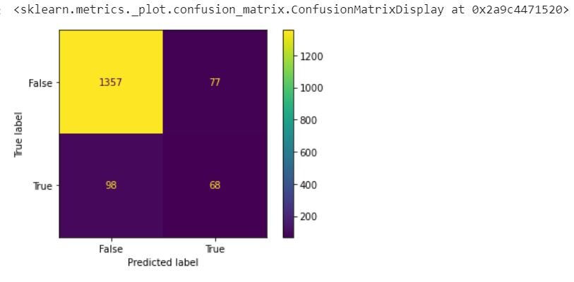
confusion_matrix(y_test,base_pred)

array([[1357,   77],
       [  98,   68]], dtype=int64)

plot_confusion_matrix(model,X_test,y_test)
print(classification_report(y_test,base_pred))

               precision    recall  f1-score   support

       False       0.93      0.95      0.94      1434
        True       0.47      0.41      0.44       166

    accuracy                           0.89      1600
   macro avg       0.70      0.68      0.69      1600
weighted avg       0.88      0.89      0.89      1600
OOF! The results of this model reflects the terribly imbalanced classes that exist. To no surprise, the model is very accurate in regards to predicting which leads won’t close and terrible at predicting the leads that will close. It would be very unwise to use the overall accuracy score of 0.89 (89%) given that there is a biased preference by the model to predict that a lead will not close. All this said, we can try to see if a very basic Support Vector Classifier will be a more balanced model.
Feature Importances:
pd.DataFrame(index=X.columns,data=model.feature_importances_,columns=['Feature Importance']).sort_values(by=['Feature Importance'],ascending=False)
Using Grid Search, an optimized Support Vector Classifier was built to determine the best parameters possible for the basic model:
from sklearn.model_selection import GridSearchCV

svm = SVC()
param_grid = {'C':[0.01,0.1,1],'kernel':['linear','rbf']}
grid = GridSearchCV(svm,param_grid)

# Note again we didn't split Train|Test
grid.fit(X,y)
After the Grid Search is complete, we can find the best parameters for the model to baseline:
grid.best_score_

0.9486120231394622

grid.best_params_

{'C': 0.1, 'kernel': 'linear'}
Not a terrible score! But, as we noted above, we need to break down this accuracy numbers into manageable components. We can do this by, first, building the simple model using the parameters found in the Grid Search:
model = SVC(kernel='linear', C=0.1)

model.fit(X_train, y_train)

y_pred = model.predict(X_test)
After the model has been trained, we can now see the accuracy for the second model we built:
print(classification_report(y_test, y_pred))

                precision    recall  f1-score   support

       False       0.96      0.98      0.97      1434
        True       0.83      0.63      0.72       166

    accuracy                           0.95      1600
   macro avg       0.89      0.81      0.84      1600
weighted avg       0.94      0.95      0.95      1600
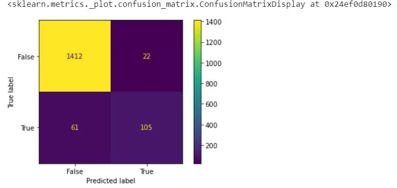
Based off this classification report above, the Support Vector Classifier performs significantly better than the Tree Based methods above—especially in the area of predicting the leads that will eventually close. There is nearly a 30% increase in the prediction accuracy of True while maintaining a high level of accuracy on False. A confusion matrix helps further contextualize accuracy:
plot_confusion_matrix(model,X_test,y_test)
Conclusion:
Initial modeling seems to indicate that the Support Vector Classifiers are better predictors than the Tree Based methods
Accuracy, especially for this use case, needs to be balanced across the True and False—especially if the data will continue to be imbalanced in the future
There are opportunities to leverage other features that were part of the original dataset, but had poor data quality. Assuming the data quality could be improved, there would be increased opportunities to improve business outcomes
Opportunities & Future work:
The imbalanced nature of the dataset should be addressed through oversampling, weighting, and attempting to use gradient boosted algorithms
Prediction of the time to close will likely be another worthwhile venture, especially when attempting to predict future sales, prioritizing lines of business, and even resource planning
Thorough discussion would need to occur between those that would use something like this in process and those that have designed the algorithm itself—industrialization would need to be done with care and monitored closely over time

